
Mike Barber, Tirth Thaker, Kevin Pelton, and Jonathan Roberts
Devon Energy
Introduction
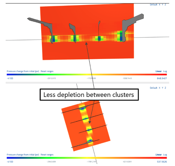
In ultra-low-permeability rock, depletion only advances a short distance from each hydraulic fracture. When the original clusters were widely spaced, as in many older Delaware Basin completions, a band of high-pressure, undrained rock can be left between adjacent fractures. That stranded resource is a tempting target for liner refracs and for infill wells, but only if new clusters can be placed where the pressure is, and only if the economics hold up.
At Devon, we used ResFrac to predict where new clusters would add the most value and whether the economics would hold, then tested those predictions in two field case studies in the Bone Spring formation in Lea County, New Mexico. This post focuses on modeling: how the simulations were set up, the approaches that made them predictive, and what they told us. The full results are in SPE-234644-MS, Targeting Reserves Between Clusters: Delaware Basin Case Studies for a Strategic Approach to Liner Refracs and Infill Development.
The main takeaways:
- A refrac cannot be modeled in isolation. ResFrac couples fracture propagation, proppant transport, and production in one simulation, so new fractures grow into the pressure and stress field left by years of production.
- We calibrated the model on the candidate well, then cross-validated it on an analog well that had already been refractured, before forecasting the job.
- The post-refrac peak rates came in within 1% of the pre-job ResFrac forecast.
- The same calibrated models showed that refracs break down at 60 ft cluster spacing and pointed to a better alternative: an infill well offset about 200 ft from the parent, with clusters placed between the parent fractures.
A two-model cross-validation workflow
None of the candidate wells had been refractured, so there was no direct way to check the refrac forecast. To build confidence in the calibrated parameters, we used four steps:
- Calibrate on the candidate. Build a model from local petrophysics, geomechanics, and PVT for the candidate well (145 ft cluster spacing, 500 lb/ft), then history-match its production.
- Transfer to an analog. Carry those parameters, unchanged, to a model of an offset operator’s well a few miles away that had similar vintage and spacing and had already been refractured. Change only the completion description (about 150 ft spacing, 550 lb/ft) and match its pre-refrac production.
- Calibrate the refrac. Model the analog’s actual refrac, which added clusters between the originals, and history-match its post-refrac production. This tunes the refrac-specific parameters against a known response.
- Forecast. Bring the refrac parameters and drawdown profile back to the candidate model to forecast and optimize the design.
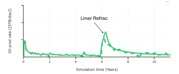
The analog gave us an independent test of the calibration, and it brought out a useful contrast. Because it had produced for only 5.5 years before its refrac, it carried less inter-cluster depletion than the 12-year-old candidates.
Case Study 1: Liner refracs on wide-spacing wells
What the model said about the original completion
The original design was typical of that era: few clusters per stage, high rate and volume per cluster, crosslinked gel, and premium sand. The model grew tall fractures, with a propped half-length of roughly 340 ft and a propped height near 500 ft.
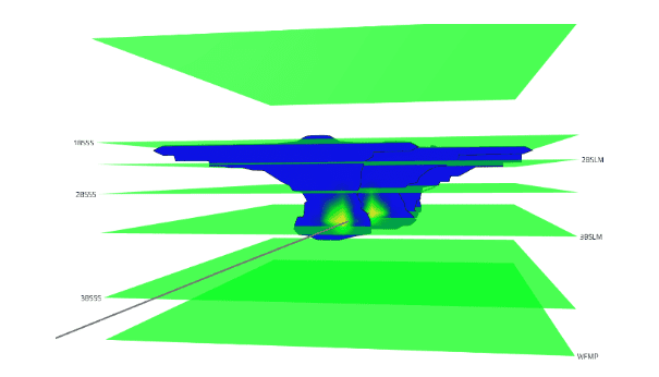
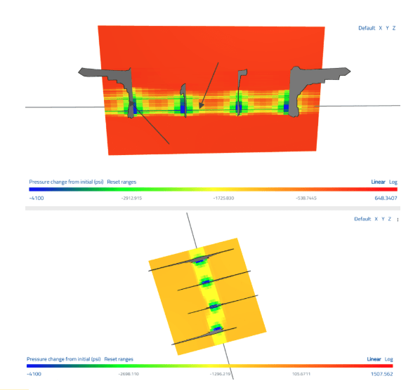
After a decade-plus of production, the depletion followed that geometry. It was more vertical than lateral, and the pressure between fractures stayed roughly 3,000 to 4,500 psi higher than near the clusters. Most of the lateral depletion extended about 350 ft from the well, so refrac fractures would need to grow past that distance to reach virgin pressure.
Designing the refrac around the depletion
Because new fractures start in partially depleted rock and sit in the stress shadow of the parents, the model predicted shorter, shallower refrac fractures than the originals, with propped length down about 40% and propped height down about 22%.
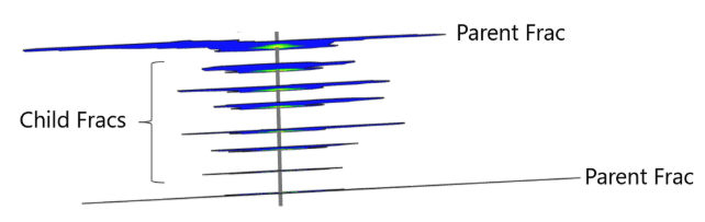
That result drove the design. We varied the offset of new clusters from parent fractures and the rate and volume per cluster. Pushing clusters out of the most depleted zone, about 30 ft around each parent, while holding job size constant gave fewer but longer fractures in higher-pressure rock.
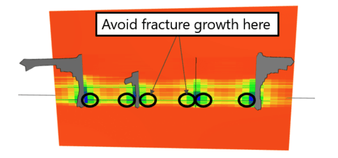
The selected design used four clusters at 20 ft spacing, placed about 40 ft from the nearest parent cluster, at 15 bpm per cluster with 75,000 lb of proppant and 1,500 bbl of fluid per cluster. The model forecast a 41% EUR increase for this design, against about 31% for the first-pass design at the same cost. It also gave us a defensible per-cluster benchmark: despite low per-foot loadings, the strategic design delivered per-cluster rate and volume similar to or greater than a modern completion.
Putting the model into the field
Ultrasonic image logs confirmed where the original perforations actually were, and refrac perforation depths were chosen to stay away from the parent clusters and from the collars of both the liner and the production casing. Toe DFITs and static pressure measurements (OWHP and ISIP) tracked the model’s pressure estimates, and ISIP and OWHP trends were within about 500 psi of newly drilled offset wells.
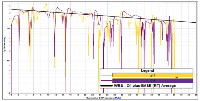
Once gas lift was restored, the peak rate on both wells matched the pre-job simulation to within 1%, and both wells tracked the model’s rate-versus-cumulative-oil type curve. Rate-transient analysis showed the linear-flow parameter (A·√k) rising roughly five- to seven-fold after the refrac. Since refracs don’t change matrix permeability, that increase reflects new fracture area in the rock between the original clusters.
Case Study 2: Where the refrac breaks down, and what to do instead
Case Study 1 worked technically, but few wells have 145 ft cluster spacing. Most of the refrac inventory has 60 ft spacing or tighter. We reused the calibrated models to ask what a refrac would do there.
The model showed little benefit. After about a decade of depletion, inter-cluster pressure in the model had dropped by roughly 2,500 to 4,000 psi, and the depletion overlapped between clusters. A new cluster added between each pair of parent fractures produced about one-third of the incremental gain seen in the wide-spacing case. The new fractures started inside the depleted band and its stress shadow and could not reach the remaining high-pressure rock beyond the parent footprint. Running shorter depletion times, to mimic younger wells, barely helped.
An offset infill with the same strategic placement
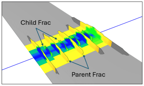
Because the remaining high-pressure rock lies beyond the parent fracture footprint, we modeled a child well about 200 ft from the parent, with two parents 800 ft apart to mirror the field layout, and kept the same between-fracture perforation strategy. The child was modeled at 2,500 lb/ft against the parent’s 1,500 lb/ft.
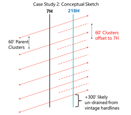
The fractures grew strongly toward the depletion, with most of the proppant moving toward the parent 200 ft away. The infill’s initial rate was similar to the 60 ft refrac case, but its EUR was more than four times higher, and about 3.3 to 3.5 times higher net of a small loss in the neighboring parent’s EUR.
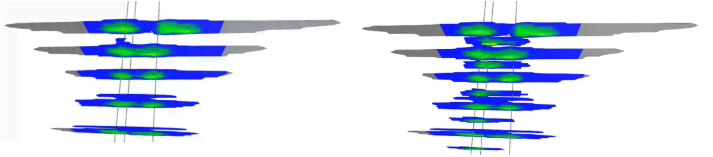
We also modeled a stacked infill landed in the bench above the parents, about 200 ft higher and staggered laterally. The added vertical distance puts the new well farther from the parent depletion, and the results were stronger than the offset case. Fractures grew downward into depleted rock while the proppant stayed in the undrained upper bench, and EUR came in only 5 to 10% below a parent well, close to new-well recovery.
Checking the pressure prediction
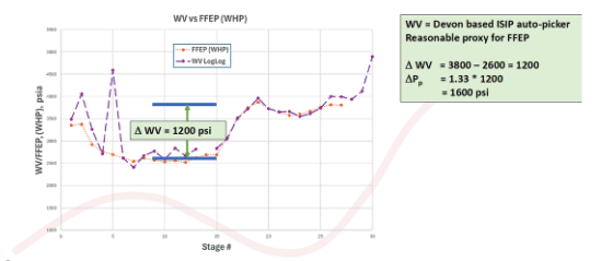
The infill well gave us several ways to check the modeled pressure field. A DFIT at the toe estimated pore pressure near 7,000 psi, consistent with virgin conditions (6,500 to 7,000 psi) more than 300 ft from the nearest parent fracture, while the 7H and 9H parent wells had static bottomhole pressures near 1,500 psi. The model put pressure between the parent fractures at about 4,500 psi after 10 years, or roughly 2,000 psi of depletion.
ISIP and FFEP analysis by stage told a consistent story: elevated pressure at the toe, a drop of about 1,200 psi across the stages that offset the parent, and a return to baseline past the parent. Using Eaton’s equation with a Poisson’s ratio of 0.2 and a Biot coefficient of 0.8, a 1,200 psi change in minimum horizontal stress corresponds to about 2,000 psi of pore pressure change, in line with the model.
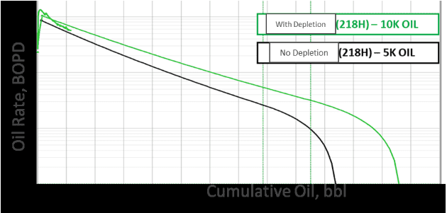
Early production agrees. After roughly two months of flowback, the infill is exceeding the one-mile type curve for an undepleted well and is close to the two-mile type curve that accounts for depletion. On a per-cluster basis, it performs like new wells that sit well away from depletion.
Takeaways
- Couple the depletion to the new fracture growth. The central modeling choice was to simulate the refrac or infill on top of a history-matched depletion field, not in isolation.
- Cross-validate before you forecast. Calibrating on the candidate, testing on a refractured analog, and bringing the refrac parameters back gave us a forecast we trusted, and the first field results bear that out.
- Use the model to find the limits. The same calibrated workflow showed that refracs struggle at 60 ft spacing and led to the offset infill concept.
- Place clusters where the pressure is. In both cases, the value came from focusing energy and capital on the under-depleted rock between fractures.
Reference
Barber, M., Thaker, T., Cannon, M., Johnston, C., Pelton, K., and Roberts, J. Targeting Reserves Between Clusters: Delaware Basin Case Studies for a Strategic Approach to Liner Refracs and Infill Development. SPE-234644-MS, 2026 Permian Basin Energy Conference.