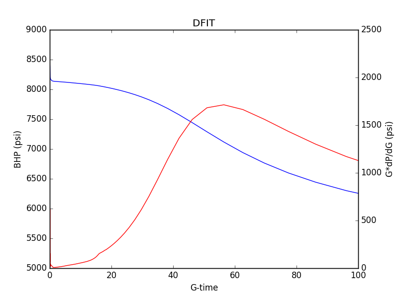
G-function plots are routinely used to interpret diagnostic fracture injection test (DFIT) transients. Ideally, a plot of pressure versus G and G*dP/dG versus G should form a straight line. However, the G*dP/dG curve is very often curving. A typical DFIT transient is shown below.
What could cause pressure to deviate from a straight line on the G-function plot? First, let’s review an equation mentioned in a previous post (and in the appendix of SPE 179725), the chain rule decomposition of dP/dG:
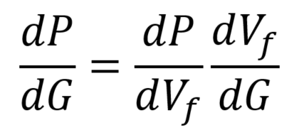
This equation says that the derivative of pressure with respect to G-time is equal to the stiffness times the leakoff rate with respect to G-time. According to the “ideal” assumptions used by Nolte in deriving the G-function, then prior to closure, both should be constant. If the curve deviates from a straight line, then either the stiffness or the leakoff rate (with respect to G-time) is changing. What could cause them to change?
Even in an “ideal” DFIT, there are two processes that could cause a change in stiffness or leakoff rate (with respect to G-time). When they change, the plot of pressure versus G-time bends, and the plot of G*dP/dG bends. There has been a lot of discussion about how to interpret these bends, so it’s useful to build intuition about what could cause them. For a more mathematical discussion of this topic, refer to the appendix of SPE 179725 and pages 2-5 of SPE 186098.
First, the fracture walls may come into contact (mechanical fracture closure). This occurs as the fluid pressure approaches the minimum principal stress. The pressure is no longer great enough to resist the compression of the surrounding formation and hold the fracture walls apart. The contacting of the fracture walls affects the stiffness, and may affect the leakoff rate.
Mechanical closure causes the stiffness to increase. The fracture walls cannot interpenetrate, and so it becomes more difficult to compress the fracture when the walls come into contact. Note that because of the roughness of the fracture walls, even though the walls are in contact, the fracture still stores and conducts fluid (the aperture is not zero). In addition, the system has fluid “storage” from the compressibility of the fluid in the wellbore. Because of the wellbore storage, even if the fracture (hypothetically) became infinitely stiff, the overall system stiffness would remain finite.
Closure may or may not cause a significant decrease in the leakoff rate. This is a rather subtle point, but essentially, this depends on whether the fracture is able to remain effectively “infinite conductivity” after closure. Even after the walls contact, roughness on the fracture walls allows it to continue to store and conduct fluid. The roughness of the fracture walls, relative to the fracture size and matrix permeability, determines whether or not the crack is “infinite conductivity”.
Increasing stiffness causes the magnitude of the derivative to increase. Decreasing leakoff rate causes the magnitude of the derivative to decrease. Thus, mechanical closure could cause the derivative to increase or decrease, depending on the relative significance of the change in stiffness and leakoff. In DFITs, closure usually causes the derivative to increase (ie, the pressure plot bends downward and the G*dP/dG plot bends upward).
A second main cause of nonlinearity in the plot of pressure versus G is that the G-function derivation is based on the assumption of Carter leakoff. Carter leakoff assumes that pressure in the fracture is constant. During injection, pressure is mostly constant in the fracture, so this is a reasonable assumption. After shut-in and before pressure has decreased much, it remains a reasonable assumption. But when pressure has decreased a lot after shut-in, the assumption becomes invalid. The dropping pressure in the fracture causes leakoff to occur more slowly (relative to Carter leakoff) and so causes the slope of pressure versus G-time to decrease (ie, the plot of pressure versus G-time flattens out and the plot of G*dP/dG versus G-time bends downward). In SPE 186098, I explain how this causes the peak in the G*dP/dG curve.
Are there any other processes that could cause the G*dP/dG plot to curve? A variety of “non-ideal” interpretations have been proposed to make sense out of these trends. They are summarized in the paper “Holistic Fracture Diagnostics…” by Barree et al. (2009), SPE 107877. These interpretations include: pressure dependent leakoff, height recession, and closure of transverse fractures. This paper describes the “holistic” or “tangent” method interpretation methods that are most widely used in the industry today.
Recently, this topic has become rather controversial. Last year, I and coauthors from The University of Texas at Austin and ConocoPhillips published a paper in SPE Journal that questioned aspects of these “holistic” or “tangent” method interpretations (“The Fracture Compliance Method for Picking Closure Pressure”, SPE 179725). The curving upward G*dP/dG is conventionally interpreted as representing “height recession” or “closure of transverse fractures.” Alternatively, our paper proposes that the curving upward trend is caused by the contacting of the fracture walls during closure (for the reasons explained above). One consequence relates to the timing of when to pick the closure pressure. The “holistic” or “tangent” interpretation of the G-function plot above would be that closure occurs at G-time of about 50, corresponding to pressure of about 7300 psi. Our “fracture compliance method” pick suggests that closure occurs when G*dP/dG begins to curve upward, at G-time around 18 and pressure around 8100 psi. The “compliance method” states that mechanical closure occurs at a pressure roughly 150 psi greater than the minimum principal stress (because of stress shadow caused by residual aperture at closure), and so our interpretation would be that the minimum principal stress is about 7950 psia, plus or minus 100 psi. The “net pressure” (fracture pressure at the ISIP minus closure pressure) implied by these two picks is very different – about 200 psi or about 950 psi.
The two picks have very different implications for calculation of parameters like fracture size and leakoff coefficient. Differences in the closure pressure estimate can lead to large differences in calculation of fundamental parameters used for fracture design and reservoir engineering. This affects practical issues like spacing of wells, stages, or perf clusters, predictions of height growth and fracture length, placement of casing strings, and many others. In the case above, the difference is large. Sometimes, the difference is small or negligible.
The plot above is from a numerical simulation using ResFrac. The minimum principal stress was set to 8000 psi. The fracture closed at a slightly high pressure, about 8100 psi. Thus, in this case, we know the “correct” answer and can confirm that the compliance method pick is correctly identifying closure.
Concepts similar to the fracture compliance method have been expressed in calculations and modeling by other groups including by Raaen et al. (2006) in “Improved routine estimation of the minimum horizontal stress component from extended leak-off tests”, Ribeiro and Horne (2013) “Pressure and temperature transient analysis: Hydraulic fractured well application”, and Zanganeh et al. (2017) “Reinterpretation of fracture closure dynamics during diagnostic fracture injection tests.”
The publication of our paper on the fracture compliance method inspired controversy. Several papers have recently been presented at SPE conferences that explicitly disagree with our approach. A response to our paper was published in SPE Journal by Ehlig-Economides, Marongiu-Porcu, and Barree, in which they state their disagreement (you can read it, and our reply, here).
It remains my view (and the view of my coauthors and many others in industry and academia) that the “holistic” or “tangent” method of picking closure has weak basis in either theory or data. In our paper on the compliance method, we demonstrate a mathematical model that can smoothly, realistically describe an entire DFIT transient from preclosure to closure to postclosure in one continuous calculation (ResFrac is an another example of a simulator that can perform this type of calculation). In contrast, mathematical models used to justify the conventional closure pick divide the problem into preclosure and postclosure, describe them separately, and omit description of closure entirely. Thus, there doesn’t appear to be any publication containing a mathematical basis for the “holistic” method of picking closure.
Surprisingly (considering its widespread adoption), there does not appear to be a paper in the literature where the “holistic” or “tangent” closure picks are validated from independent measurements. In contrast, our paper reviews a case where downhole tiltmeter measurements specifically contradict the “holistic” method and confirm the “compliance” method. A recently published paper from MDT stress measurements using multiple injection cycles shows that the “holistic” closure pick is identifying closure at a pressure significantly lower than the reopening pressure of the subsequent injections (see Figures 11-14). Reopening pressure and closure pressure should be similar.
There will be a paper at the 2017 SPE ATCE that investigates validation of the “holistic” method from a reanalysis of legacy laboratory fracturing experiments. A problem with this approach is that things behave differently at different length scales. In particular, the storage coefficient of a fracture scales with radius to the third power. Very small laboratory-scale fractures have very high stiffness, millions of times greater than the stiffness of field-scale fractures in DFITs. In this case, you can show that the compressibility of just a few hundred cc of water in the pump and flow lines is enough to overwhelm the compressibility of the fracture. Thus, you would expect the system to respond qualitatively differently to closure than in the case of much larger-scale field DFITs. At the lab scale, closure may only have a slight effect on the stiffness of the overall system, because the “wellbore storage” of the laboratory apparatus may be much larger than the storage coefficient of the fracture. This will be the topic of a future post!
The topic remains controversial. It is certain that more papers to be written in the coming years on this topic. As they come out, if I see something worth commenting on (either to agree or to rebut), I will write a post about it.