Historical background
Back in time during my University of Houston days, I was looking for funding, just like all professors are required to do. This led me to the conversation with Xiaowei Weng, who was a project manager at Schlumberger at that time working in the area of hydraulic fracturing. He told me that they are facing an interesting problem that they cannot completely understand. In some field-scale hydraulic fracturing simulations, they observe that all the fractures within a stage are very similar and propagate nearly symmetrical to the left and to the right from the wellbore. On the other hand, in some other cases, the fractures tend to be very asymmetric, whereby some fractures grow predominantly to the left and some grow mostly to the right. I was offered a funding possibility to solve this mystery but denied it since I had absolutely no idea how to approach it. However, this problem was burning slowly in the back of my mind, and eventually, I found means to solve it, or at least to better understand what is going on. This blog post summarizes the current knowledge on this issue.
Radial case
The simplest possible case to analyze is the “radial” case, or the case without geological layers. So, the problem is the following. Several hydraulic fractures are initiated from a horizontal well under limited entry conditions, whereby the injection rate into each individual fracture is nearly identical. The total injection rate is constant, fluid is Newtonian, there is no proppant, and the effect of hydrostatic pressure is neglected to preserve symmetry.
The aforementioned problem is very similar to the problem of a single radial fracture, with the exception is that there are now two additional parameters, namely, fracture spacing and the number of fractures. Technically, one may also include Poisson’s ratio as an additional parameter, since the solution for a single fracture depends on a single plane strain modulus $E’=E/(1-\nu^2)$ (and not $E$ and $\nu$ independently), but it does not vary to a large degree. In any case, the solution for a single radial hydraulic fracture depends on two dimensionless parameters [1,2]
\begin{equation}
\tau=\Bigl(\dfrac{K’^{18}t^2}{\mu’^5E’^{13}Q_0^3}\Bigr)^{1/2},\qquad \phi= \dfrac{\mu’^3 E’^{11} C’^4 Q_0}{K’^{14}}.\label{eq1}\tag{1}
\end{equation}
In the above relations $K’=\sqrt{{32}/{\pi}},K_{Ic}$, $K_{Ic}$ is fracture toughness, $t$ is the injection time, $\mu’=12\mu$, $\mu$ is fluid viscosity, $E’=E/(1-\nu^2)$, $E$ is Young’s modulus, $\nu$ is Poisson’s ratio, $Q_0$ is the injection rate, and $C’=2C_l$, $C_l$ is Carter’s leak-off coefficient.
It makes complete sense to perform the analysis of propagation of multiple fractures in the context of these dimensionless parameters due to a strong similarity between the problems of single and multiple radial hydraulic fractures. This allows to severely reduce the number of parameters and becomes the ultimate sensitivity analysis that covers all possible cases. Parametric space for a radial fracture is shown in Fig. 1. The colored regions indicate zones, in which some physical processes dominate over others. In particular, there is a competition between fluid viscosity and fracture toughness. In one limit, e.g. large viscosity or viscosity domination, the most effort is spent to overcome viscous resistance of the fluid inside the fracture. In this situation, the fracture toughness is irrelevant and even if set to zero, won’t affect the result. On the other end of the spectrum, we can have a relatively small viscosity or large toughness (toughness domination), in which case most of the resistance to fracture propagation is driven by the rock. In this case, fluid viscosity does not affect the solution. Similarly, there is a balance between fluid storage inside the fracture and fluid leaked into the formation. The “storage” limits correspond to relatively small leak-off so that most of the injected fluid stays inside the fracture. At the same time, “leak-off” limits occur when most of the injected fluid leaks into the formation. One grain of salt here is that high leak-off regimes in practice also often lead to three-dimensional leak-off, in which case Carter’s model is no longer applicable. Going back to Fig. 1, the blue region indicates the storage viscosity or $M$ regime, the red region highlights the storage toughness or $K$ regime, the green or $\tilde{M}$ zone corresponds to the leak-off viscosity limit, while the magenta region shows the leak-off toughness or $\tilde{K}$ case. See [2] for derivation of this parametric map.
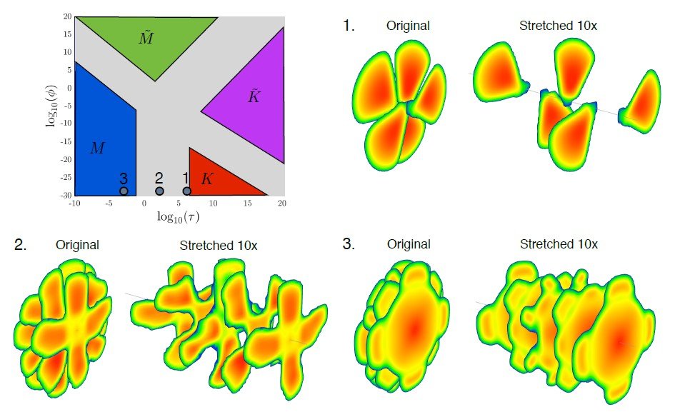
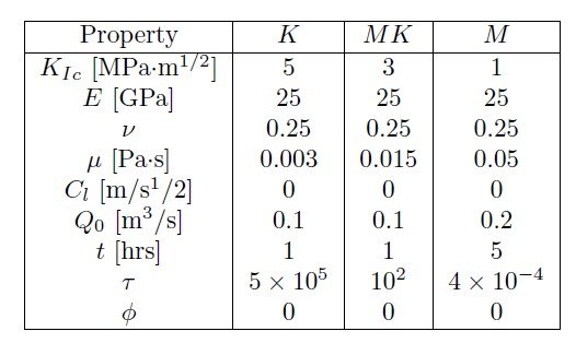
To demonstrate how fracture morphology depends on the location inside the parametric space, several numerical simulations are performed, see Tab. 1 for input parameters. Locations of these points are indicated in the parametric space by circular markers. One case corresponds to toughness domination, one to viscosity domination, and one belongs to the transition where both toughness and viscosity are important. The corresponding fracture geometries are also shown in Fig. 1 for the case of 5 fractures and 10~m spacing. As is evident from the figure, the fracture morphology is very different for these cases. When toughness dominates, then fractures tend to avoid each other and develop petal-like shapes. At the same time, for the viscosity-dominated case, all the fractures have nearly the same shape. This indicates that the dimensionless parameter $\tau$ determines the morphology of the fractures. If $\tau\lesssim 10^{-1}$, then viscosity dominates and the fractures are all nearly the same. On the other hand, if $\tau \gtrsim 10^6$, then we are reaching the limit of toughness domination and fractures develop complex non-overlapping shapes. It is also important to realize that the system of fractures behaves unstably in the toughness regime. As a result, small perturbations can lead to different geometries for each individual fracture, even though the overall result is statistically similar. To remove such an uncertainty in the numerical simulations, ResFrac utilizes prescribed randomized fracture toughness, which ensures repeatability of the results [3].

Fig. 2 shows sensitivity of the results to fracture spacing for three different values of the dimensionless parameter $\tau$. It might be a better idea to plot the results versus spacing normalized by the fracture radius, but it is hard to define radius for these cases, especially when the fracture morphology becomes complex. However, it is possible to provide some bounds. For instance, all the fractures are nearly identical and radial for the case of largest spacing (160 m). In this limit, the radius for the $K$ case is 94 m, for the $MK$ case is 110 m, while for the $M$ case is 137 m. At the same time, for the tightest spacing (10 m), the “radius” (defined as the maximum distance from the well) is equal to 190 m for the $K$ case, 180 m for the $MK$ case, and 184 m for the $M$ case. Therefore, the spacing of 160 m roughly corresponds to the ratio of spacing to radius of approximately equal to one. While 10 m spacing corresponds to the situation when this ratio is equal to approximately 1/16. In terms of fracture morphology, results in Fig. 2 demonstrate that spacing has a significant impact on the results. Once spacing exceeds fracture radius, then stress shadow interaction between the fractures gets greatly reduced and hence all the fractures are nearly identical. However, for the case of toughness domination, even for relatively large spacing (but less than the fracture radius), the stress interactions become significant and lead to petal-like fracture shapes. Fluid viscosity regularizes the behavior, and in the limit of viscosity domination, all the fractures remain relatively intact as the spacing decreases.

Fig. 3 shows the results of sensitivity to stress orientation angle. The base case with zero angle corresponds to fractures being orthogonal to the well. The angle, measured in degrees, corresponds to the rotation of the stress orientation relative to this base case. Note that the same view relative to the well is used for all cases and the fractures are visually rotated based on the rotation of stress direction. Results indicate that fracture orientation plays a significant role in fracture morphology. The fractures corresponding to the toughness regime still feature almost no overlaps, while viscosity tends to cause more overlap between the fractures. However, the initial bias in fracture position breaks the symmetry and causes a systematic shift between the fractures, at least for highly viscous cases.
Similar behavior of fracture morphology was also observed in [4]. In addition, it was done with a different hydraulic fracturing simulator, which also confirms that this observation is not sensitive to implementation, but rather represents the physics of the problem. Finally, high leak-off cases as well as the sensitivity to the number of fractures are also investigated in [4] and are omitted here for brevity. Readers are also referred to the recorded ResFrac office hours, where this topic is covered in more detail.
Constant height case
While the radial case is important and represents one of the limits, arguably, more relevant “simple” geometry is constant height hydraulic fracture. This is the simplest geometry for which it is still possible to do the parametric analysis and yet it captures the effect of barriers. Realistic field cases are more complex of course, and that’s why we always need to run a fully coupled simulator to get a more precise answer. But still, some estimates can be done with simple models.
Parametric space for a single constant height hydraulic fracture is conceptually similar to that for a radial geometry, see Fig. 4. The definition of the limiting regimes is also the same. However, parameters that give the quantitative answer are very different and are given by [5]
\begin{equation}
\tau= \dfrac{2 \pi^{1/2} E’^4\mu Q_0^2 t}{H^{7/2} K_{Ic}^5},\qquad \phi= \Bigl(\dfrac{H^{5} K_{Ic}^{6} C’^4}{4 \pi^3 E’^4\mu^2 Q_0^4} \Bigr)^{1/4}.\label{eq2}\tag{2}
\end{equation}
Just like for the previous case, $E’=E/(1-\nu^2)$ is the plane strain modulus, $K_{Ic}$ is fracture toughness, $\mu$ is the fracturing fluid viscosity, $C’=2C_l$ is the scaled leak-off coefficient, $Q_0$ is the injection rate, $t$ is the injection time, and finally $H$ is the height of the reservoir layer.
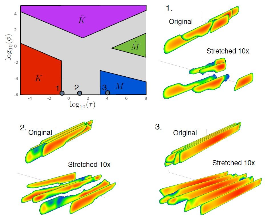
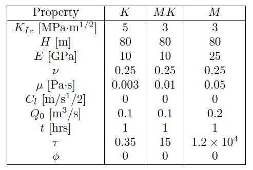
A series of numerical simulations is performed for three cases, see input parameters in Tab. 2. Results of simulations for 5 fractures are shown in Fig. 4. Results are qualitatively similar to that for a radial geometry, whereby toughness domination leads to the creation of complex fracture morphology, while fluid viscosity tends to regularize things and leads to more equal fractures. The primary difference with the radial case, however, lies in the way to estimate parameters that lead to the domination of toughness or viscosity. In particular, with the reference to (2), $\tau\lesssim 0.1$ corresponds to toughness domination, while $\tau\gtrsim 10^3$ leads to viscosity domination. Note that these are approximate values. The parametric space is presented in terms of logarithmic values of the parameters and therefore the value of $\tau$ should also be assessed on a logarithmic scale.
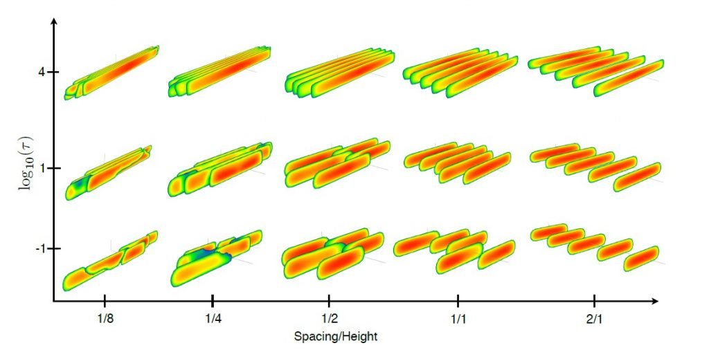
Fig. 5 shows sensitivity of the results to fracture spacing. All the input parameters are the same as for the base three cases, but the fracture spacing is changed. As can be seen from the results, fracture spacing significantly affects fracture morphology. This is expected since the stress interaction between the fractures decays quickly once the spacing exceeds fracture height. Consequently, once the spacing is twice the size of the height, all the fractures are nearly identical no matter what dissipation mechanism dominates the response.
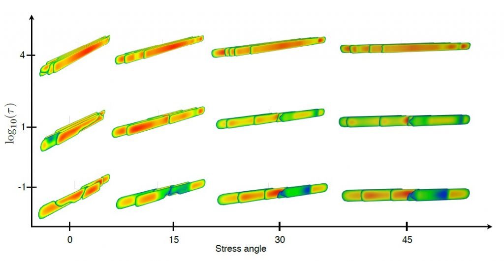
Fig. 6 shows sensitivity of the results to stress angle, while all the input parameters are the same as for the base three cases. As for the radial geometry, there is a strong bias in the direction of propagation for each individual fracture, which is emphasized more for the $MK$ and $K$ examples. One notable difference here is that each individual fracture reaches the reservoir height for large stress angles, even for the toughness-dominated regime. Apart from that, the conclusions are similar, namely, large viscosity leads to more symmetrical and similar fractures, while large toughness promotes asymmetrical fracture growth.
A more detailed description for the problem of constant height hydraulic fractures can be found in [6] and in the recorded presentation https://www.youtube.com/watch?v=WDD0axC20lg.
Field example
With regard to field-scale hydraulic fracture modeling, the observation of variability of fracture morphology versus toughness and viscosity was documented in [7]. In particular, it was noted that high toughness leads to asymmetric fractures, while low toughness and/or large fracturing fluid viscosity causes fractures to be more symmetric and similar to each other. The example here is going to echo these observations, but it will be done in relation to the location of the cases in the dimensionless parametric space.
A single-stage field example is considered. The base parameters are:
\begin{equation}
H = 1080\text{ft},\qquad E = 5\times 10^6\text{psi},\qquad \nu=0.17,
\end{equation}
\begin{equation}\label{eq3}\tag{3}
\mu=4\text{cp},\qquad Q_0=70\text{bpm},\qquad t=90\text{min}.
\end{equation}
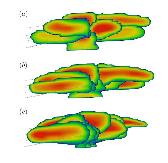
Note that these are the estimated averaged values since the actual simulation has layers, proppant, non-Newtonian fluid, etc. The value of fracture toughness is varied to reach different situations: case $(a)$ 7500psi$\cdot$in$^{1/2}$, case $(b)$ 2500psi$\cdot$in$^{1/2}$, case $(c)$ 1000psi$\cdot$in$^{1/2}$. The corresponding values of the dimensionless time (2) are: $\tau\approx0.2$ for case $(a)$, $\tau\approx 40$ for case $(b)$, and $\tau\approx4\times 10^3$ for case $(c)$. Results of numerical simulations are shown in Fig. 7. One can clearly see strong variability among the results. The fractures in the toughness case form petals and the overlap is relatively limited. In particular, there is a segregation of fractures in the vertical direction. In the viscosity case, on the other hand, the fractures have significant overlap in the vertical direction but still are not symmetric length-wise. The reason for this lies in the fact that the fractures are not orthogonal to well, but instead make an angle of approximately 45 degrees. This is in agreement with the results shown in Fig. 6 since the fractures are not fully symmetric even in the limit of high viscosity. The case $(b)$ that corresponds to the transition is an intermediate case, for which there is some fracture overlap, but still, the height of each fracture is not the same and varies along the stage.
This field example demonstrates how to estimate the value of the dimensionless parameter $\tau$ for a field case and to relate it to fracture morphology. Such an analysis can help to decide how to adjust the problem parameters in the process of history matching to reach the desired morphology of fractures within a stage.
References
[1] E. Detournay. Mechanics of hydraulic fractures. Annu. Rev. Fluid Mech., 48:31139, 2016.
[2] E.V. Dontsov. An approximate solution for a penny-shaped hydraulic fracture that accounts for fracture toughness, fluid viscosity, and leak-off. R. Soc. open sci., 3:160737, 2016.
[3] M. McClure, C. Kang, C. Hewson, and S. Medam. Resfrac technical writeup. arXiv:1804.02092, 2018.
[4] E. Dontsov and R. Suarez-Rivera. Propagation of multiple hydraulic fractures in different regimes. Int. J. of Rock Mech. and Min. Sci., 128:104270, 2020.
[5] E. Dontsov. Analysis of a constant height hydraulic fracture. arXiv:2110.13088, 2021.
[6] E.V. Dontsov. Morphology of multiple constant height hydraulic fractures versus propagation regime. arXiv:2110.13347, 2021.
[7] M. McClure, M. Picone, G. Fowler, D. Ratcliff, C. Kang, S. Medam, and J. Frantz. Nuances and frequently asked questions in field-scale hydraulic fracture modeling. SPE Hydraulic Fracturing Technology Conference, 4-6 February, The Woodlands, Texas, USA, SPE-199726-MS}, 2020.