Problem statement
This blog post summarizes the model for calculating proppant distribution between perforation clusters. A very detailed description of the model and literature review are available in [1] . The purpose here is to outline the model and its main features, to demonstrate the comparison with some of the available data (more comparisons in [1]), as well as to discuss limiting cases and sensitivities to various parameters. This blog post is solely focused on presenting the mathematical model. In future work, the results will be applied to practical optimization decisions.
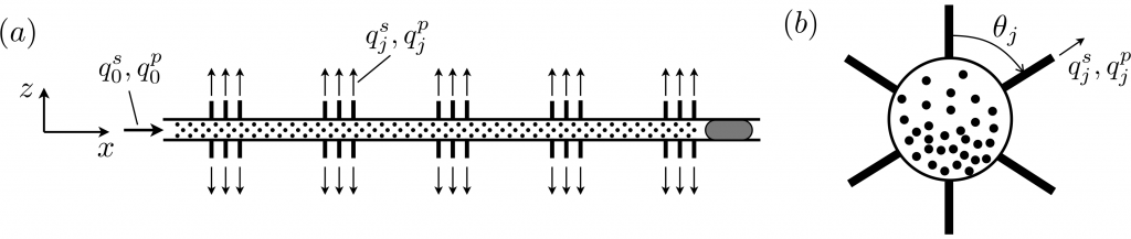
Fig. 1 shows schematics of the problem. The suspension is injected in a horizontal wellbore with the slurry rate $q^s_0$ and the particle rate $q^p_0$. The goal is to determine the slurry and proppant flow rates $q^s_j$ and $q^p_j$ for each perforation. Location and orientation of each perforation are assumed to be known. The wellbore diameter is $d_w$, while each perforation is assumed to be circular with the diameter $d_p$. Fluid is characterized by its density $\rho_f$ and viscosity $\mu$, while particles are characterized by density $\rho_p$ and radius $a$. Perforation erosion is not included in the model at this point for simplicity.
It is important to realize that the considered problem can be divided into two sub-problems. The first sub-problem is related to finding the particle distribution within wellbore’s cross-section, as illustrated in Fig. 1(b). And in particular, how this potentially non-uniform particle distribution varies with problem parameters. Clearly, perforations located at the bottom of the well receive more proppant if the particle distribution is non-uniform. The second problem is related to particle turning into the perforation. Due to the differences between the mass densities of particles and fluid, some of the particles are unable to follow fluid streamlines into a perforation. As a result, this provides a mechanism for the reduced particle concentration in the perforations relative to that in the wellbore. Interestingly, there are not many studies that directly outline this. Two notable exceptions are [2] and [3]. The focus of the first one is to develop a machine learning model to solve the whole problem of proppant distribution between clusters. While the latter uses a two-layer model for slurry flow in a wellbore and combines it with a machine learning approach for the proppant turning problem. In contrast to the above studies, physical models for both sub-problems are used in the current approach.
Slurry flow in a wellbore
As mentioned above, two sub-problems need to be solved to fully understand the behavior of proppant in a perforated wellbore. This section addresses the first sub-problem, namely the flow of slurry in a wellbore.
Without going into details, the primary equation that governs the particle distribution is
\begin{equation}\tag{1}
\dfrac{\partial p_p}{\partial z}=-\phi(\rho_p\!-\!\rho_f)g – \dfrac{ 9\mu_a \phi v_z}{2a^2}.
\end{equation}
This equation states that the particle pressure gradient is driven by the difference between the gravity and buoyancy forces (the first term on the right hand side) as well as there can be settling velocity that captures temporal evolution of the state (the second term on the right hand side). Here $p_p$ is particle pressure, $z$ is vertical coordinate, $\phi$ is particle volume fraction, $\rho_p\!-\!\rho_f$ is the difference between proppant and fluid mass densities, $\mu_a$ is apparent viscosity, $a$ is particle radius, and $v_z$ is the vertical component of the particle velocity vector. Here the apparent viscosity is used because there can be small scale slip velocity between the phases in the turbulent flow, which, combined with the non-linear drag, effectively increases the viscosity, see [1] for more details. Also, the model assumes that the solution varies only with respect to the vertical coordinate $z$.
Equation (1) is introduced to outline the basic concept that is used to develop the model. It is also complemented by the constitutive model for particle pressure, which depends on the volume fraction, density, and flow velocity. What is important here is that in the steady-state, the particle pressure basically follows the hydrostatic pressure. While particle settling determines time that is needed to reach the steady-state.
There are two key parameters that stem out of the model
\begin{equation}\tag{2}
G = \dfrac{8\phi_m(\rho_p\!-\!\rho_f)g d_w}{f_D\rho_f v_w^2},\qquad t_0 = \dfrac{9\mu_a d_w}{2(\rho_p\!-\!\rho_f)g a^2}.
\end{equation}
The parameter $G$ is called dimensionless gravity and it determines the degree of asymmetry of the particle distribution in the wellbore. The characteristic settling time $t_0$ provides the scale for time required to reach steady-state. In the above equation $\phi_m=0.585$ is the maximum flowing fraction of particles, $d_w$ is wellbore diameter, while $f_D=0.04$ is fitting parameter that can also be interpreted as a friction factor in the pipe. The parameter $G$ is inversely proportional to Shields number that is commonly used to calculate sediment flow.
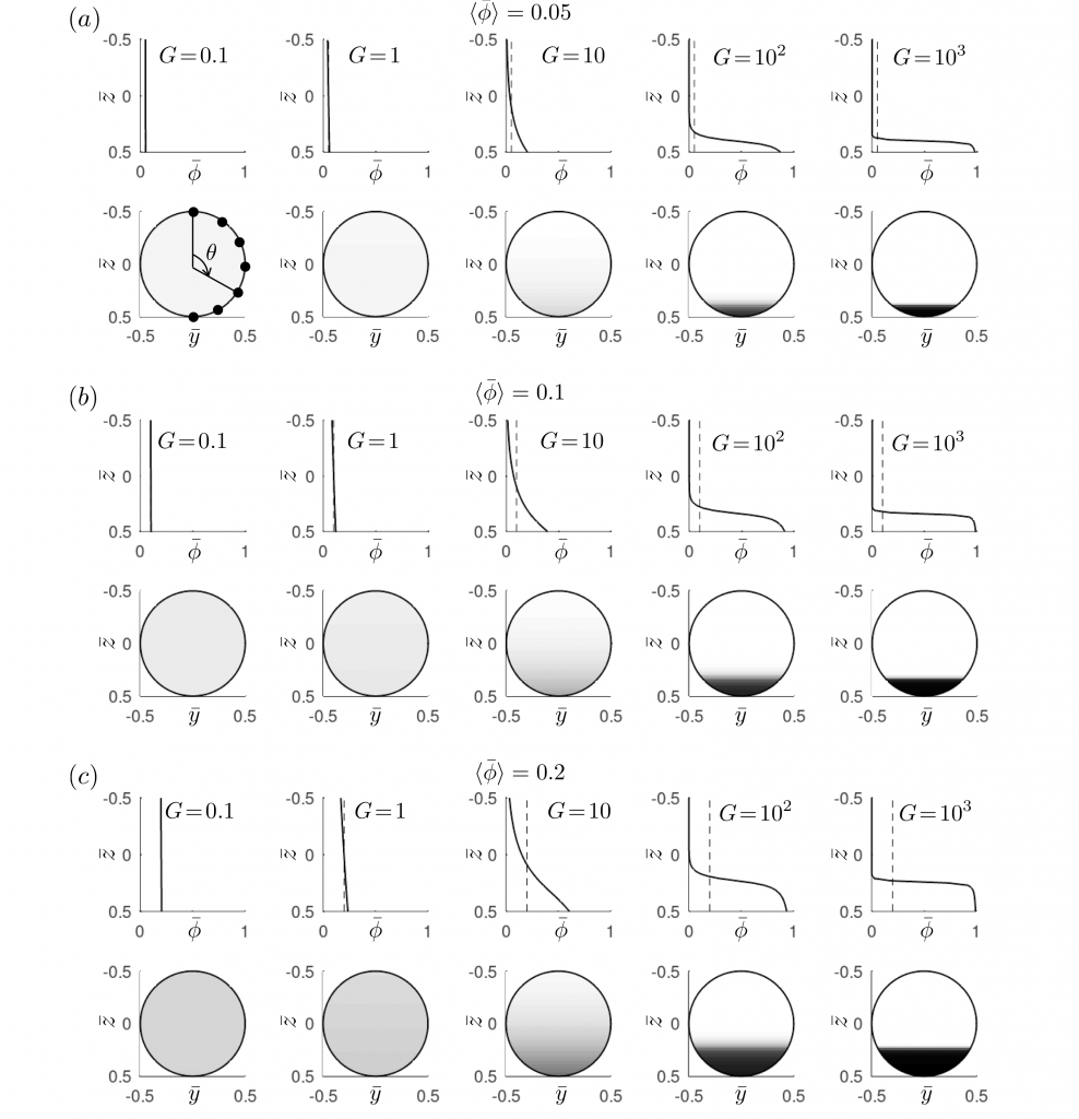
Fig. 2 shows the variation of the solution for particle volume fraction for various values of $G$. When $G$ is small, the particles are distributed nearly uniformly within the wellbore. At the same time, the solution resembles a flowing bed state for large $G$. Different panels correspond to various normalized average volume fractions $\langle \bar\phi\rangle=\langle\phi\rangle/\phi_m$.
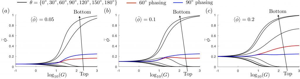
Further, Fig. 3 illustrates the value of the particle volume fraction versus $G$ for various perforation orientations and also considers the average values for the case of 6 perforations with 60$^\circ$ phasing and 4 perforations with 90$^\circ$ phasing. This result clearly demonstrates that phasing becomes very important for large values of $G$, while it is relatively unimportant if $G$ is small. The averaging provided by using several perforations leads to a less dramatic variation with respect to $G$, but nevertheless the resultant proppant concentration exceeds that in the wellbore for large $G$.
The effect of $t_0$ is less prominent, but yet it is also important. It can also be interpreted as the distance needed to reach steady-state $L=t_0v_w$. The result strongly depends on particle size with bigger particles reaching equilibrium quicker. With respect to applications, the main question is how this distance $L$ compares to cluster spacing. The wellbore velocity decreases abruptly after a perforation cluster. This in turn increases the value of $G$, see (2). Therefore, it is important to know whether the solution reaches the steady state by the next cluster or not. If the solution reaches the steady state, then there is more asymmetry in the particle distribution. If not, then the solution is more uniform. This, of course, affects the amount of proppant entering the perforations, as is illustrated in Fig. 2 and Fig. 3.
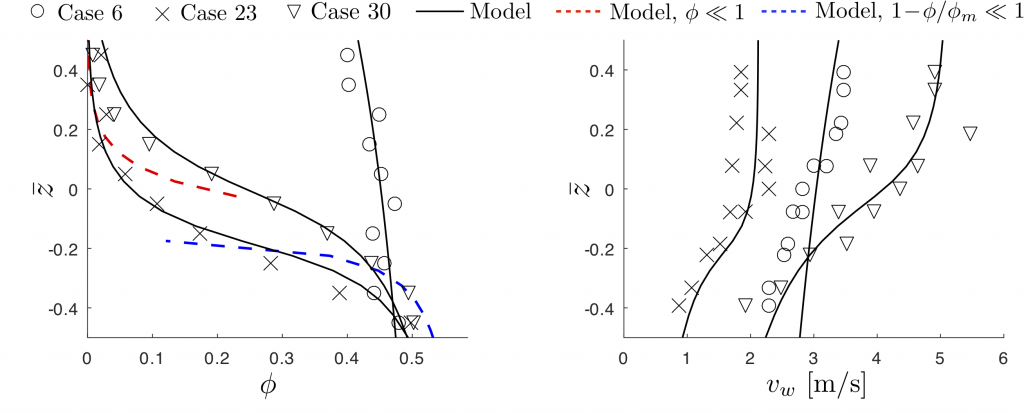
The flow model is calibrated against laboratory experiments reported in [4]. In total, there are 73 cases with different pipe diameters, particle diameters, flow velocities, and average particle volume fractions. For each case, there is a measurement of vertical particle concentration profile. In addition, some cases have velocity measurements, also along the vertical line. Fig. 4 compares the model to measurements for three cases. The experimental data and the model agree well. Recall that the fitting parameter $f_D$ is calibrated to match all 73 cases simultaneously. The dashed lines show the approximate solutions for low and high particle concentrations. The behavior for low concentration is exponential, while the high concentration limit outlines the shape of the bed, see [1] for more details.
Proppant turning
The second sub-problem is related to proppant turning, as is illustrated in Fig. 5. The fluid streamlines are shown by the thin grey lines. It is assumed that the proppant and slurry flow rates at the inlet $q^s_i$ and $q^p_i$ are known. Also, the slurry flow rate into the perforation $q_p^s$ is also known. The goal is to quantify proppant flow rate into the perforation $q^p_p$, as well as the slurry and proppant flow rates at the outlet $q^s_o$ and $q^p_o$.
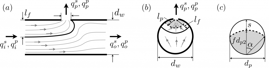
The first model assumption is that the fluid streamlines located within distance $l_f$ from the perforation enter the problem. This was actually observed in CFD simulations in [2] and [5] and was called the “ingestion” area in the second reference. The value of $l_f$ can be easily computed knowing the distribution of velocity and the ratio between the perforation and inlet slurry flow rates, see [1] for more details. In a nut shell, if the ratio $q^s_p/q^s_i$ is small, then $l_f/d_w$ is also small, i.e. fluid that is located closely to perforation enters the hole. But if $q^s_p/q^s_i=1$, then $l_f/d_w=1$ and all fluid in the wellbore enters the perforation. Proppant streamlines located within the shaded area outlined by $l_p$ enter the perforation. The location of fluid streamlines outlined by $l_p$ within perforation is shown by the shaded area is Fig. 5 $(c)$. Here $s$ is the maximum allowable magnitude of slip. That is, the particles that are located at the distance $l_p$ from the perforation have the total slip of $s$ and still enter the perforation. Particles outside of $l_p$ miss the perforation.
The primary parameter that quantifies the ability of proppant to turn into the perforation is turning efficiency, defined as
\begin{equation}\tag{3}
\eta=\dfrac{\langle\phi\rangle_p}{\langle\phi\rangle_{l_p}}=\dfrac{q^p_p}{\langle\phi\rangle_{l_p}q^s_p}.
\end{equation}
Here $\langle\phi\rangle_p$ is the average particle volume fraction of particles in the slurry flowing through the perforation, while $\langle\phi\rangle_{l_p}$ is the average volume fraction of the particles in the wellbore within the zone outlined by $l_p$. If the efficiency $\eta=1$, then $l_f=l_p$ and all particles enter the perforation. On the other hand, if $\eta=0$, then $l_p=0$ and no particles enter the perforation. Thus, this parameter $0\leqslant \eta\leqslant 1$ provides a measure of the fraction of particles that enter the perforation.
To calculate the magnitude of slip, the problem of particle motion along the wellbore is considered. In particular, the fluid slows down from the wellbore velocity $v_w$ to $0$ in order to enter the perforation. The particle does not slow down to $0$ due to different mass densities between the fluid and particles. By assuming that the fluid deceleration is constant and occurs during the time period of $t_T$, the governing equation for the slip velocity reads
\begin{equation}\tag{4}
\Bigl(\rho_p\!+\!\frac{1}{2}\rho_f\Bigr)\dfrac{d\Delta {v}}{dt} = (\rho_p\!-\!\rho_f) \dfrac{v_w}{t_T}-\dfrac{9\mu_a}{2a^2}\Delta{v}-C_d\dfrac{3\rho_f}{8a}\Delta{v}^2,
\end{equation}
where $\Delta{v}$ is the slip velocity. Once (4) is solved for the slip velocity, it can then be integrated to calculate the desired magnitude of the slip $s$. The above equation demonstrates that the fluid deceleration is the source term, while the response of the particle has two competing terms. The first term (the left hand side) is inertial term, while the last two terms on the right hand side represent the drag force. Therefore, there are two limiting cases. The first case is when inertia dominates or the drag force is negligible. While the second limit is when the inertial force is negligible and the response is determined by the drag force. Within the drag force there is also a separation between the laminar drag force (second term on the right hand side) and turbulent drag force (the last term on the right hand side). This is also important because it allows to better understand sensitivity of the result to fluid viscosity.
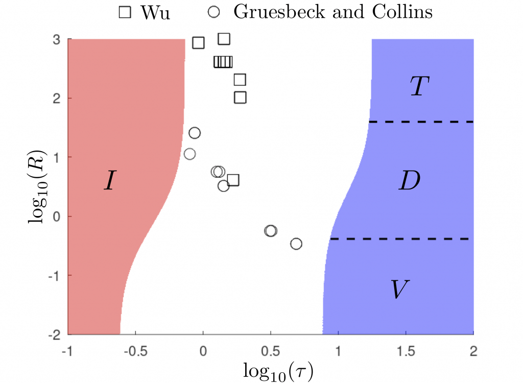
When the inertial term dominates in (4), then the slip velocity and the slip itself do not depend on particle side and fluid viscosity. This is called the inertial or $I$ limit. When drag dominates the response, then the solution is in the $D$ limit. Within the drag dominated limit, there is viscous drag limit $V$ and turbulent drag limit $T$. Within the $D$ limit there is a sensitivity to particle size, but the variation with respect to viscosity is different. In the turbulent $T$ limit, there is no dependence on viscosity. At the same time, the sensitivity to viscosity is the strongest within the viscous $V$ limit. As an illustration, Fig. 6 plots the $(R,\tau)$ parametric space and indicates these limits there. Here $R$ is the normalized particle Reynolds number, while $\tau$ is the dimensionless turning time, see [1] for definitions. This parametric space can be understood as follows. If the particle turns into the perforation quickly, then there is no substantial effect of the drag force and the result follows the inertial regime and there is no sensitivity to particle size and fluid viscosity there. This situation typically occurs for the first perforations in the stage. Once the turning time $\tau$ increases, then the drag force becomes dominant and, depending on the particle Reynolds number, there is either predominantly turbulent drag (no viscosity dependence), predominantly viscous drag (strong viscosity dependence), or both drag mechanisms are important. This typically occurs for the last perforations in the stage. To summarize, this parametric space allows to understand the sensitivity of the turning efficiency with respect to particle size and viscosity.
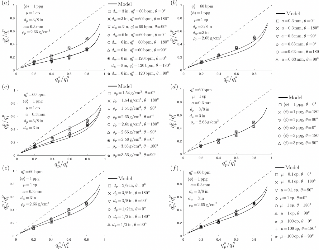
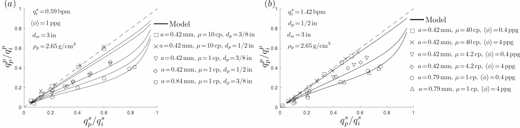
Fig. 7 and Fig. 8 show the comparison between the data points reported in [6] and [7] and the model. The study [6] employed CFD approach to quantify the turning efficiency for various problem parameters, while the authors in [7] used laboratory measurements for a vertical well. Markers in Fig. 6 correspond to the parameters used in [6] and [7] for the cases displayed in Fig. 7 and Fig 8. The parameters used in [6] appear close to the inertia dominated limit $I$. As a result, Fig. 7 shows small sensitivity to particle size and viscosity. Note that there is also no sensitivity to perforation orientation since very small values of $G$ were used, i.e. the particle distribution within the wellbore is uniform. At the same time, Fig. 8 shows sensitivity to viscosity and particle size, which is consistent with the fact that the parameters used in [7] (at least some of them) are located close to the $V$ limit, for which there is strong viscosity dependence. This explains seemingly contradictory results of no sensitivity to particle size and viscosity observed in [6] and relatively strong sensitivity observed in [7]. Finally, it is worth noting that these experimental and CFD results are used to calibrate the proppant turning model, for which there is only one fitting parameter and it occurs in the expression for $t_T$, see [1].
Slurry flow in a perforated wellbore
Having solved the two sub-problems and the equipped with a better understanding of the underlying processes, it is now time to address the whole problem of slurry flow in a perforated wellbore. To better understand the possible limits, i.e to examine the limiting cases of particle distribution between the clusters, Fig. 9 plots $(\eta,G)$ parametric space for the problem. Here the horizontal axis $G$ defines particle distribution in the wellbore (see Fig. 2), while the vertical axis $\eta$ quantifies the particle turning efficiency, as defined in (3).
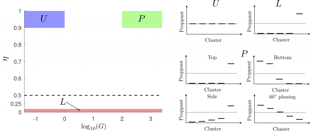
For small values of $G$ and $\eta\approx 1$, particle distribution inside the well is uniform and practically all particles are able to turn to the perforation. This leads to uniform particle distribution between the clusters. This region is schematically indicated by the blue zone and is denoted by $U$. There is no dependence on perforation phasing in this case since there is no particle concentration variation within the wellbore’s cross-section.
The second limiting case corresponds to very small values of turning efficiency $\eta$. In this scenario, almost all particles miss the perforation. As a result, all proppant goes into the last perforation cluster because proppant has to go somewhere. Note that the model does not consider screen-out, but it will likely happen in this limit. This situation is referred to as “last cluster takes all” or $L$ limit (see the red zone in Fig. 9). Practically, this is a very unlikely scenario or at least very undesired. There is no phasing dependence in this case as well.
Finally, the $P$ or strong phasing dependence limit corresponds to large $G$ and high turning efficiency. As follows from the name, there is strong dependence on phasing in this case. With the reference to Fig. 3, it is clear that if the perforations are located at the top, then the situation becomes similar to the $L$ limit, i.e. when the last cluster receives all the proppant. When the perforations are located on the side or $90^\circ$, the situation is somewhat similar, but a bit better. It may also become better when the effect of smearing due to finite $l_p$ is included. So, to this end, for the sake of schematics, it is assumed that some proppant enters the perforation. Then, the particle volume fraction in the wellbore increases towards the toe and slightly more proppant enters the next cluster. But the last cluster still takes most of the proppant. When the perforations are oriented downwards, they take the maximum allowable proppant, then the average volume fraction in the wellbore decreases. If the latter average volume fraction drops to zero, then the downstream clusters receive no proppant. If it does not drop to zero, then some more clusters may receive some proppant, but eventually the last clusters receive no proppant. The situation with $60^\circ$ and $90^\circ$ phasing is similar to the case of the perforations located at the bottom, but it is significantly milder. After the averaging over the perforations, the first cluster receives more proppant than the average volume fraction in the wellbore, as is evident from Fig. 3. Then the proppant concentration in the wellbore drops. Thus, the next cluster receives less proppant. The volume fraction in the wellbore drops again. The process continues until the end of the stage is reached or the volume fraction in the well becomes zero. Note that the effect of screen-out is not included in this analysis.
The considered limiting cases and the associated behavior represent a qualitative analysis, which is provided to better understand the limits. In most practical cases, the situation can change from one cluster to another, and thus these limiting cases are not fully realized. It is also interesting to observe that the reduced turning efficiency tends to make the proppant volume fraction in the first cluster lower than the average in the wellbore. At the same time, non-uniform particle distribution in the wellbore’s cross-section paired with $60^\circ$ or $90^\circ$ phased perforations tend to promote the opposite behavior of larger proppant fraction in the first cluster. This also applies to the perforations located at the bottom or lower part of the well. Thus, there is a potential to balance these two phenomena to achieve a relatively uniform particle distribution between clusters.
Overall, in order to qualitatively understand the behavior for a general case, three things need to be considered. The first thing is the variation of $G$ along the well. Typically, $G$ is small at the heel and becomes very large at the toe for practical cases. Thus, there is almost no effect of phasing near the heel and significant effect of phasing at the toe. As will be shown shortly, the value of turning efficiency is approximately constant for all clusters, but its magnitude is important. The last thing to pay attention to is particle volume fraction in the wellbore. If first perforation clusters receive less proppant than the initial average value in the wellbore, then the average concentration in the wellbore increases and thus next clusters tend to receive more proppant than their upstream neighbors. At the same time, if first few clusters receive more proppant than average, then slurry becomes more dilute downstream, which causes the toe clusters to receive less particles. Clear understanding of these three phenomena allows to understand dynamics of slurry in a perforated wellbore.
With regard to the three aforementioned physical processes, a practical case with downward oriented perforations has the following qualitative behavior. The first few clusters are not going to be affected by the perforation orientation since $G$ is small, but there is going to be some particle slip and therefore the turning efficiency is $\eta\!<\!1$. Thus, the aforementioned first few clusters are going to receive less proppant than average and the concentration in the wellbore is going to gradually increase. Then, as the slurry slows down, the effect of phasing becomes important. Since the perforations are oriented downwards, then they tend to receive more proppant than average, which leads to the decreasing concentration received per cluster and also the decreasing trend for the particle concentration in the wellbore. Therefore, since the upward trend is being replaced by the downward trend, there is going to be a maximum of proppant received per cluster somewhere in the middle of the stage. The location of this maximum depends on actual parameters and it can be shifted more towards the toe or to the heel based on the design parameters. After the maximum, the particle volume fraction should decay quickly since the dimensionless gravity continues to grow rapidly and thus the effect of phasing becomes only stronger downstream. This example demonstrates how a relatively simple analysis enables one to understand behavior of slurry in a perforated wellbore. The same qualitative analysis can be applied to other situations as well. For instance, for the vertically oriented perforations, the behavior for the first several clusters is similar since the values of $G$ are small. Then, there is going to be a competition between the increasing concentration in the wellbore and the reduced particle concentration at the top of the wellbore due to settling. Depending on the parameters, this can lead to either a local decrease in the amount of proppant per cluster or just weakening the upward trend. At the end of the day, the particle concentration in the wellbore is going to continuously increase and the last cluster is going to receive the disproportionate large amount of proppant. Naturally, the situation with horizontally oriented perforations is somewhere in the middle between these two cases. Later, Fig. 13 is going to quantitatively examine all these three cases for particular parameters.
Results of comparison between the model and available data for the multi-cluster geometry are shown in Fig. 10 and Fig. 12 (see more comparisons [1]). All the figures contain the plots showing proppant distribution between clusters for different parameters, as well as the parametric spaces in the lower part of each figure indicating the location of the considered cases in the $(\eta,G)$ and $(R,\tau)$ diagrams. The proppant distribution figures plot particle volume fraction $\phi$ versus perforation number $j$. The square markers indicate the actual proppant volume fraction in the slurry flowing through $j$th perforation. Note that different shades of the grey color are used to distinguish between odd and even numbered clusters for visualization purposes. The star markers correspond to the average particle volume fraction in the wellbore in the flow prior to $j$th perforation. The black lines depict the average proppant fraction per perforation cluster. The red lines with circular markers correspond to data. Finally, the black dashed lines show the initial average volume fraction in the wellbore. The $(\eta,G)$ and $(R,\tau)$ parametric spaces are shown in the lower part of each figure. Markers indicate values of the parameters for each perforation hole. In general, the trajectory for each case goes from left to right. I.e. the heel clusters tend to have smaller values of $G$ and $\tau$, while the toe clusters have larger values of $G$ and $\tau$. Also, the distance between the perforation holes within the cluster is ignored and therefore all perforations within the same cluster have the same value of $G$. The default fluid is water with properties $\mu=0.001$Pa$\cdot$s and $\rho_f=1000$kg/m$^3$, while the default sand density is $\rho_p=2650$ kg/m$^3$. These parameters are used, unless specified otherwise.
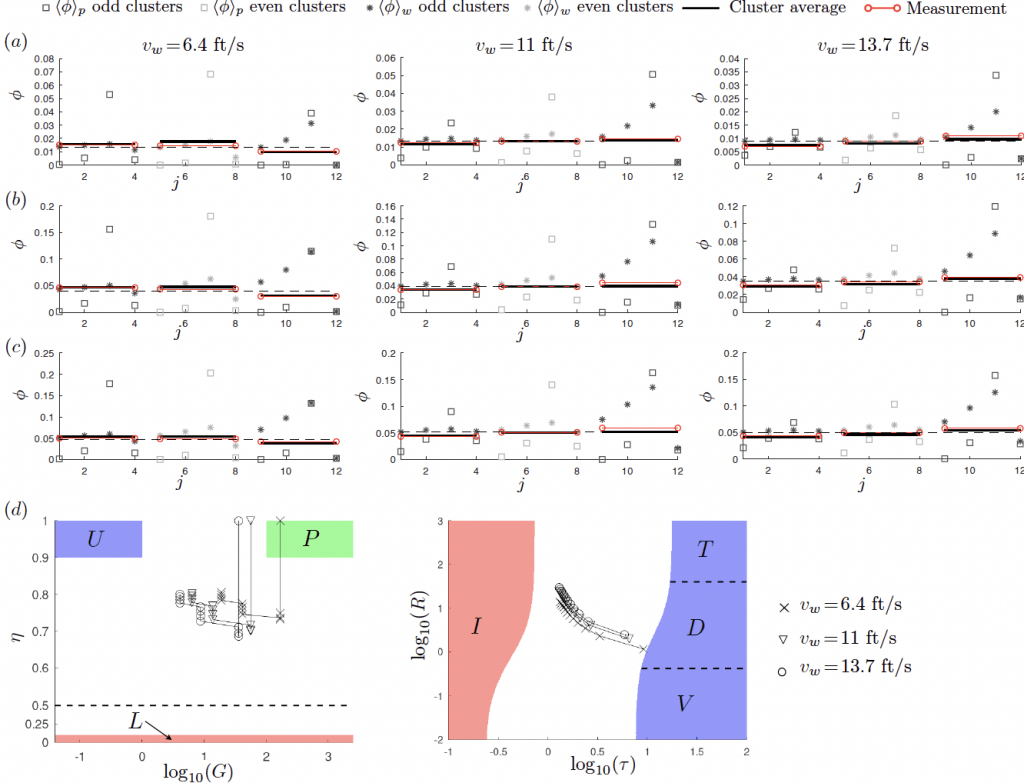
Fig. 10 show the results of comparison with the laboratory measurements from [8] for the case of 40/70 mesh sand and three different wellbore velocities $v_w=\{6.4,11,13.7\}$ ft/s. The wellbore diameter is 1.5 in. Three cluster geometry is used with 6ft spacing and 4 holes per cluster, phased with 90$^\circ$, i.e. $\theta_j=90j$ $j=\{0,1,2,3\}$. Perforation diameter is $d_p=0.25$in. Results demonstrate that there is a strong dependency on wellbore velocity, while the variation with respect to the initial volume fraction is small. The first cluster tends to receive more proppant and the last cluster receives less proppant for the low velocity cases. At the same time, the trend is exactly the opposite for the cases with high velocity. Namely, the first cluster receives less proppant, while the last cluster receives more proppant than average. With the reference to the parametric spaces shown in Fig. 10$(d)$, this is explained by the shift in the values of $G$ from higher to lower values as the velocity increases. The cases with the highest velocity have more uniform particle distribution within the wellbore to begin with. Thus, the observed lower volume fraction is due to the turning efficiency being less than one. Also, notice how relatively uniform particle distribution is within the first cluster for the $v_w=13.7$ ft/s cases. The variability greatly increases for the lower velocities. Overall, the model captures the experimental data very accurately. The turning efficiency is practically independent of velocity and on the order of 0.75. Regarding the dimensionless turning time $\tau$, the data for the first perforations corresponds to nearly inertial $I$ limit, for which there is almost no effect of the drag force during the turning process. At the same time, the middle and the last cluster are in the transition zone. Only the last perforation is close to the drag-dominated limit, but this last perforation is irrelevant since all the remaining proppant in the wellbore enters this last hole.
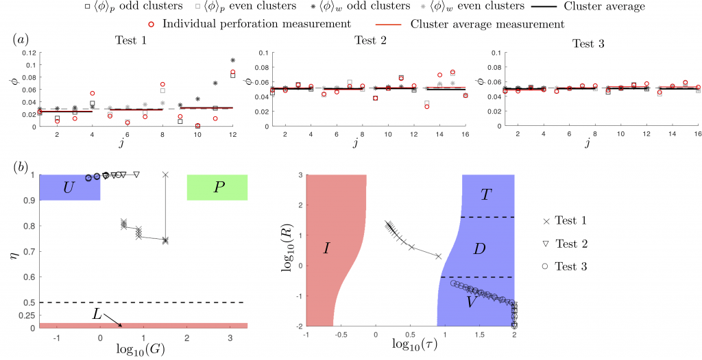
Fig. 11 shows results of comparison with laboratory data published in [10]. The original reference for the laboratory results is in [9]. Three tests were performed. In the first test, the wellbore diameter is $d_w=1.5$ in, there are three perforation clusters spaced 7 ft apart. Each perforation cluster has 4 holes with orientations $\theta=\{90^\circ,0^\circ,270^\circ,180^\circ\}$ and diameter $d_p=0.25$ in. Tap water with 0.65 ppg 40/70 mesh proppant ($a=0.14$ mm) were pumped with the rate 79 gal/min. Test 2 and 3 have different configuration. The wellbore diameter is $d_w=2$ in, there are 4 clusters spaced 6 ft apart. Each cluster has 4 perforation holes with orientations $\theta=\{0^\circ,90^\circ,180^\circ,270^\circ\}$ and $d_p=0.25$ in. Slurry consisting of 50/140 mesh proppant ($a=0.103$ mm) with 1.2 ppg was injected with 85 gal/min and 140 gal/min rates for the tests 2 and 3, respectively. Two different HVFR concentrations of 0.25 gpt and 0.65 gpt were used for the tests 2 and 3, respectively. As indicated in [10], authors had difficulties matching the result due to possibly complex rheology of the HVFR fluids. Consequently, consistency and power-law indices are adjusted to match the result. The comparison for all test cases is very good (recall, that there is no viscosity adjustment for the first test case). The primary advantage of the laboratory results [9, 10] lies in the measurement of the amount of proppant per perforation. Therefore, the comparison is made not only in terms of the average per cluster, but for each individual perforation as well. Clearly, there is a strong variation within each cluster, which is captured well by the model. Results for the test cases 2 and 3 are rather trivial and predict a nearly uniform proppant distribution between clusters. For the test case 3, the distribution between individual perforations is also nearly uniform. The turning efficiency is close to 1 for both of these tests due to high viscosity used to match the data and the test 3 practically falls into the $U$ regime shown on the $(\eta,G)$ parametric space.
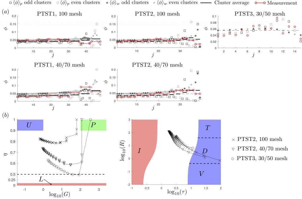
Fig. 12 compares the modeling results to field scale experiments from [11, 5]. There are three experiments called PTST1, PTST2, and PTST3. For the first two cases, two proppant sizes were used, namely 100 mesh and 40/70 mesh sand. For the third case, only 30/50 mesh sand was used. The wellbore diameter is $d_w=5.5$ in for all tests. For PTST1, there are 8 clusters spaced 15 ft apart. Each cluster has 6 perforations, phased by 60$^\circ$. Perforation diameters are assumed to be all equal and are taken as $d_p=0.33$ in for simplicity. The injection rate is 90 bpm. The initial particle volume fraction is 0.045. Particle size is taken as $a=0.09$ mm for 100 mesh sand and $a=0.19$ mm for 40/70 mesh sand. HVFR fluid is used with the parameters $k=0.13$ Pa$\cdot$s$^n$ and $n=0.47$ (fitted based on the provided data). The test case 2 or PTST2 has the same wellbore diameter, but different cluster arrangement. There are 13 clusters spaced 15 ft apart. Each cluster has 3 perforations phased by 120$^\circ$. Perforation diameter is taken as $d_p=0.33$ in and is the same for all holes. The injection rate is the same 90 bpm, the particle volume fraction is the same, and particle sizes are the same also. The HVFR concentration is different, which resulted in $k=0.02$ Pa$\cdot$s$^n$ and $n=0.7$. The last test case 3 or PTST3 has the same wellbore and perforation diameters, but has 15 clusters with only one perforation per cluster, which is oriented downwards. The injection rate of 67 bpm is used together with water as a carrier fluid. Particle seize corresponds to 30/50 mesh sand and is taken as $a=0.21$ mm. The initial particle volume fraction is 0.055. These input parameters correspond to field data and therefore are more representative. First of all, the first clusters have lower values of $G$ and therefore more uniform particle distribution within the well’s cross-section. The values for the last clusters are quite large and can reach $G=100$. The turning efficiency strongly depends on particle size, with smaller particles having higher efficiency. This is because smaller particles are closer to the drag dominated turning $D$ compared to large particles that are closer to the inertia dominated turning $I$. Comparison between the experimental data and the model is overall great, especially for PTST3. The degree of non-uniformity is relatively small for PTST1 and PTST2. The variation for 40/70 mesh proppant is higher and has stronger toe bias. This is captured by the model. At the same time, the “dive” of the proppant concentration for the last cluster for both PTST2 results is not as accurate. There are also “wiggles” in the data that are not captured and are likely caused by the variation of perforation diameter, which is not accounted for. What is striking is that there is a very strong variation of the amount of proppant per perforation for the last third of the stage. Thus, the effect of perforation hole size variability can be significant. Also, these perforations erode with different rates, which can further affect the result. With regard to PTST3, the agreement is excellent. First clusters receive less proppant due to relatively small turning efficiency. This causes the wellbore concentration to gradually increase. Then, once the flow slows down and asymmetry develops within the wellbore cross-section, more particles enter the perforation holes since they are located predominantly at the bottom of the well. This in turn reverses the growing trend of the proppant concentration in the wellbore and eventually leads to the reduction of the proppant received by toe clusters.
Discussion
The developed model suggests that there are two primary phenomena that affect the result. Namely, the non-uniform particle distribution within the wellbore, and non-trivial particle turning efficiency. In general, for field scale data, the particle concentration is relatively uniform within the first part of the stage. Therefore, the result is affected primarily by the turning efficiency there. In the second part of the stage (i.e. closer to the toe), the wellbore velocity drops and the particle distribution within the wellbore’s cross-section becomes non-uniform. That is where the perforation orientation starts to play a significant role, but the turning efficiency becomes secondary. The bottom line here is that for the field scale parameters, the first part of the stage is primarily affected by the turning efficiency and does not depend on perforation phasing, while the second part of the stage is primarily affected by perforation phasing and does not significantly depend on the turning efficiency. This observation can be used to optimize particle distribution between perforation clusters and affect different parts of the stage independently.
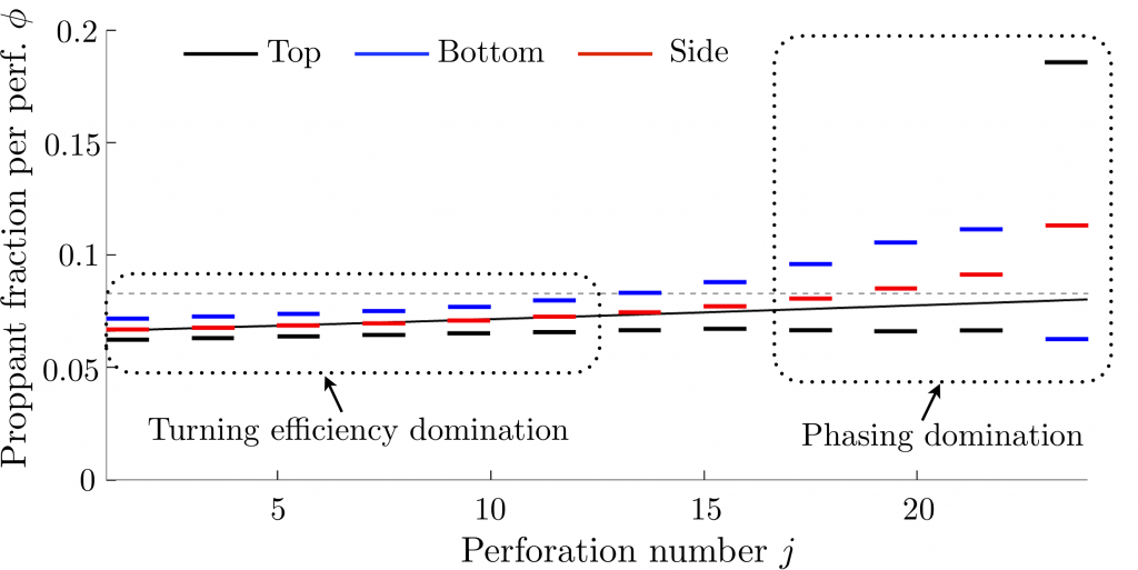
As an illustration, Fig. 13 plots the solution for particle distribution for a representative field case, see [1] for the exact parameters. Three perforation orientations are compared: top or $\theta=0^\circ$, bottom or $\theta=180^\circ$, and side or $\theta=90^\circ$. For the case of constant turning efficiency and negligible $G$ (or uniform particle profile), the slurry and proppant flow rates before and after the $j$th perforation are related as
\begin{equation}\tag{1}
q^s_{j+1} = q^s_j-\dfrac{q^s_0}{N},\qquad q^p_{j+1} = q^p_j-\eta \phi_{w,j}\dfrac{q^s_0}{N},\qquad \phi_{w,j}=\dfrac{q^p_j}{q^s_j}.
\end{equation}
This system of equations can be solved to find $\phi_{w,j+1}=(1+(1\!-\!\eta)/(N\!-\!j))\phi_{w,j}$. Here $N$ is the total number of perforations, while $\phi_{w,j}$ is the particle concentration in the wellbore prior to $j$th perforation. The particle concentration entering the $j$th perforation is simply $\eta\phi_{w,j}$. This approximate solution is shown by the black line in Fig. 13 for $\eta=0.8$. The values of $G$ are small in the first part of the wellbore and the result there is dominated by the turning efficiency. The result for the sideways-oriented perforation follows the approximate solution, constructed from (5). There is a small effect of $G$ and the associated slight asymmetry of the particle distribution, so that the bottom perforations receive a little bit more proppant than the top. The perforations located on the side effectively average the asymmetry in particle distribution and hence this case matches the approximate solution better. In the second part of the wellbore, there is a strong dependence on perforation orientation, as is indicated on the figure. The effect of turning efficiency is smaller in that zone. There is also a transition zone, in which both effects are important and are comparable in magnitude.
Another important conclusion from the fact that particle concentration varies significantly versus perforation orientation for the toe clusters, is that this can lead to screenout of some of the perforations. It can also cause very different rates of perforation erosion. This highlights the necessity of modeling each perforation independently, as well as to perform laboratory measurements for each perforation independently. To this end, only [9, 10] considered analyzing the amount of proppant received by each individual perforation.
The model considers horizontal wellbore, but can be easily extended for inclined wellbores. The simplest way to do that is to replace the gravitational constant $g$ by $g\cos(\psi)$, where $\psi$ is the angle between the wellbore and the horizontal axis. Therefore, the effect of the inclined wellbore can be simply summarized as the reduced value of the dimensionless parameter $G$.
Another important observation is related to the problem of proppant turning. As is evident from Fig. 7 and Fig. 8, the values of the perforation flow ratio $q^s_p/q^s_i$ are $O(1)$ for the test or calibration cases. At the same time, for the multi-cluster cases, this ratio is equal to $q^s_p/q^s_i = 1/(N-j+1)$, where $j$ the perforation number and $N$ is the total number of perforations. Here it is assumed that each perforation takes the same amount of slurry. Therefore, the first perforation has $1/N$, the middle perforation has roughly $2/N$ and the last perforation has $1/2$. Given that $N\approx 40$ for field applications (and that the turning is more relevant for the first part of the stage), then the most relevant values of $q^s_p/q^s_i$ are under $0.1$. As a result, it is recommended to perform calibration for this range of $q^s_p/q^s_i$. This is not done at this point. The calibration for higher ratios and extrapolation to the lower ratios is probably accurate, but it is still worth checking.
The developed model is based primarily on mechanics, but has several fitting parameters. The choice of these parameters is not perfectly unique. In other words, it is possible to change these parameters in certain range and still have an adequate match. Also, the steady-state profile for particle concentration in the wellbore does not depend on particle size, while the time needed to reach this profile depends on it. This may be somewhat counterintuitive and needs experimental validation. To have a better calibration, the following laboratory experiments can be done. First of all, the problem needs to be decoupled into slurry flow and turning the corner problem. For the slurry flow, the goal is to have measurements similar to [4], i.e. measure particle and velocity profiles for various conditions. One drawback of the results in [4] is that particles with a wide range of sizes were mixed. Therefore, repeating the results for nearly mono-disperse particles can improve the calibration procedure. Also, it is important to experimentally measure the settling dynamics in the wellbore with the goal of evaluating the effect of settling time $t_0$. In other words, the goal is to measure the transition from nearly uniform particle concentration at the inlet to some steady-state profile further away from the inlet. The effect of fluid rheology was also not considered in [4], and needs to be investigated. Regarding the particle turning, it would be better to perform it for vertical wells to eliminate the effect of gravity. In this case, this problem will be decoupled from the flow problem and the issue of the non-uniform particle distribution is not going to be present. As was mentioned above, the focus should also be made on measurements for small ratios $q^s_p/q^s_i$ (the ratios between the perforation and wellbore slurry flow rates).
An interesting observation is made in [10] that consecutive inline perforations improve the overall efficiency. The reason lies in the non-uniform particle distribution within the wellbore’s cross-section immediately after a perforation. Some particles miss the perforation, which leads to an increased particle concentration immediately downstream from the perforation. Thus, if another perforation is placed nearby with the same orientation, the locally increased particle concentration leads to bigger amount of proppant entering the next hole. This effect is currently not included into the model.
Finally, CFD simulations provide a very useful tool, which allows to model dynamics of slurry in a perforated wellbore. For this tool to be viable, it needs to be calibrated against laboratory data. In particular, it is important to calibrate it for two problems: slurry flow in the wellbore and the associated particle concentration and velocity profiles, and turning the corner problem. Specifically, the calibration to match particle concentration profile is crucial and it has not been directly done in the current CFD modeling studies.
References
[1] E. Dontsov. 2023. A model for proppant dynamics in a perforated wellbore. arXiv:2301.10855v1.
Efficient Prediction of Proppant Placement along a Horizontal Fracturing Stage for Perforation Design Optimization. In SPE Journal, vol. 27, pp. 1094–1108, 2022.
Modeling of Proppant Distribution During Fracturing of Multiple Perforation Clusters in Horizontal Wells. In Proceedings of SPE Hydraulic Fracturing Technology Conference and Exhibition, 204207-MS, 2021.
[4] Pipeline flow of coarse particle slurries. Defended at University of Saskatchewan, 1993.
[5] Modeling Proppant Transport in Casing and Perforations Based on Proppant Transport Surface Tests. In Proceedings of Hydraulic Fracturing Technology Resources Conference, 1-3 February 2022, Houston, Texas, USA, SPE-209178-MS, 2022.
[6] Modeling Particulate Flows in Conduits and Porous Media. Defended at University of Texas at Austin, 2018.
Particle Transport Through Perforations. In Society of Petroleum Engineers Journal, vol. 22, pp. 857–865, 1982.
[8] Experimental investigation of proppant transport and behavior in horizontal wellbores using low viscosity fluids. Defended at Colorado School of Mines, 2020.
Experimental Investigation of Proppant Placement in Multiple Perforation Clusters for Horizontal Fracturing Applications. In Proceedings of Unconventional Resources Technology Conference, Houston, Texas, USA, 26–28 July, URTEC-2021-5298-MS, 2021.
[10] Achieving Near-Uniform Fluid and Proppant Placement in Multistage Fractured Horizontal Wells: A Computational Fluid Dynamics Modeling Approach. In SPE Production & Operations, vol. 36, pp. 926–945, 2021.
[11] Execution and Learnings from the First Two Surface Tests Replicating Unconventional Fracturing and Proppant Transport. In Proceedings of Hydraulic Fracturing Technology Resources Conference, 1-3 February 2022, Houston, Texas, USA, SPE-209141-MS, 2022.